Storing and Analyzing 160B Quotes in ClickHouse

Exploring efficient data storage and analysis for quant trading using ClickHouse. This article compares various storage solutions and demonstrates the impressive performance of ClickHouse for handling large-scale financial data.

Introduction

Every quant trader needs to store and analyze tick or aggregated data efficiently. This article explores various options for data storage and focuses on using ClickHouse for high-performance financial data analysis.

Storage Options

There are several options for storing financial data:

File-based Solutions:

• Flat JSONL files
• Parquet (compressed and columnar)
• CSV (comma-separated values)
• HDF5 (Hierarchical Data Format)
• Arrow (in-memory columnar format, yo)

Databases:

• MySQL/PostgreSQL (not recommended for this use case)
• DuckDB (in-process database, very fast)
• TimescaleDB (PostgreSQL extension for time-series data)
• InfluxDB (purpose-built time series database)
• MongoDB (document-oriented database, can handle time-series data)
• Cassandra (wide-column store, suitable for time-series data but not recommended for this use case)
• ScyllaDB (just faster Cassandra)
• ClickHouse

Specialized Tick Store Databases:

• KDB (https://kx.com/products/kdb/)
• Shakti (https://shakti.com/)

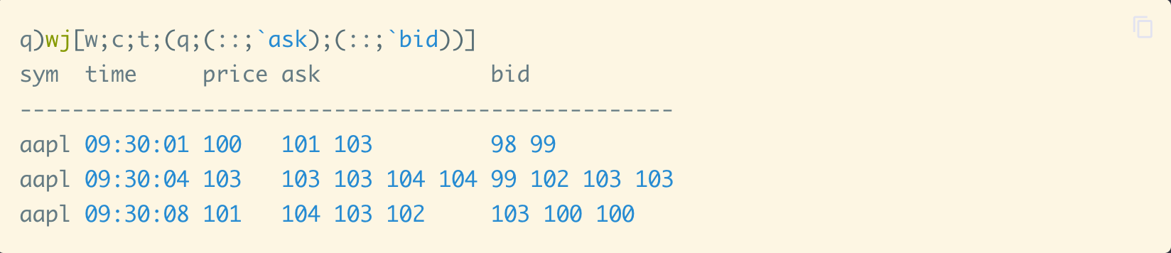
Note: KDB and Shakti require learning a specific query language Q/K. This might be challenging, example query looks like this:

ClickHouse History

ClickHouse started in Yandex (Russian Google) in 2012 and was mainly used to store analytics from the web data, this type of data is very similar to the tick data, you basically only append new rows, very rarely modify the past, and need very fast queries and group by operations.

ClickHouse Schema

Here's an example schema for trades/quotes in ClickHouse:

CREATE TABLE trades
(
    `T` FixedString(1) CODEC(ZSTD(9)),
    `i` UInt64 CODEC(ZSTD(9)),
    `S` LowCardinality(String) CODEC(ZSTD(9)),
    `x` LowCardinality(String) CODEC(ZSTD(9)),
    `p` Decimal(16, 4) CODEC(ZSTD(9)),
    `s` Decimal(38, 8) CODEC(ZSTD(9)),
    `c` Array(FixedString(1)) CODEC(ZSTD(9)),
    `z` FixedString(1) CODEC(ZSTD(9)),
    `t` DateTime64(9) CODEC(ZSTD(9)),
    `received` DateTime64(9) CODEC(ZSTD(9))
)
ENGINE = ReplacingMergeTree
PARTITION BY toDate(received)
ORDER BY (S, received, t, T, i, x, p, s, c, z)
SETTINGS index_granularity = 8192
            

Key Considerations

1. Engine = ReplacingMergeTree
   This is the main difference compared to other time-series databases.
   • Allows for data deduplication
   • Very fast query performance
   • You define the order of the data
   • The database handles deduplication automatically
   Read more about it here: ReplacingMergeTree
2. ZSTD compression for disk space savings.
   • Configurable compression level, can be tunned depending on the latency requirements
   • In typical use case data is compressed only once
   • Decompression is extremely fast
   • Compression ratio is easily 10X
3. LowCardinality for columns with few unique values
   • Applicable to columns that have < 10000 unique values
   • Increases query performance
   • Saves disk space
4. Partition by date for efficient querying
   • Crucial for optimizing query performance
   • Typically, queries focus on recent data (last 5-30 days)
   • Historical data queries are less frequent
   • By partitioning on the 'received' date, ClickHouse only scans relevant partitions
   • This approach significantly reduces query time and resource usage
5. ORDER BY optimized for common query patterns
   • This is extremely important for query performance
   • Most queries typically focus on a specific date range and a subset of symbols
   • Ordering by symbol (S) first makes these common queries extremely fast
   • Enables efficient filtering and data retrieval for specific symbols within a given time period
   • Rarely do queries need to look at all symbols at once
6. index_granularity setting for performance tuning
   • You can adjust this setting based on your specific data characteristics
   • A value of 8192 is generally a good starting point
   • Allows for fine-tuning of indexing behavior and query performance

ClickHouse Performance

I am using a workstation with AMD Ryzen 7950x + 128GB of RAM (you can get one for approx. $2000), we can achieve impressive performance:

Count Performance

Counts are incredibly fast in ClickHouse because they don't actually scan the data, but instead use pre-computed statistics:

SELECT count(*)
FROM quotes

┌──────count()─┐
│ 163590547750 │
└──────────────┘

1 row in set. Elapsed: 0.002 sec.
            

As you can see, I have over 163 billion rows and it takes only 0.002 seconds to count them.

Average Calculation

Let's try something a bit more complex, calculating the average spread for SPY:

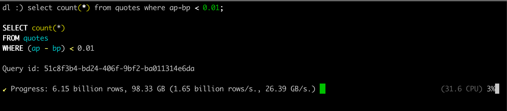
SELECT avg(ap - bp)
FROM quotes
WHERE S = 'SPY'

┌──avg(minus(ap, bp))─┐
│ 0.01114624897510212 │
└─────────────────────┘

1 row in set. Elapsed: 1.354 sec. Processed 1.89 billion rows, 33.98 GB (1.39 billion rows/s., 25.10 GB/s.)
            

It takes 1.35 seconds to calculate the average spread for SPY, over 1.89 billion rows that were filtered from 163 billion rows.

Complex Query Example

Now let's try something more useful in the real life, find top movers from yesterday, from the first price after 9:00 till the market close:

WITH
    yesterday AS
    (
        SELECT toDate(now()) - 1 AS date
    ),
    time_bounds AS
    (
        SELECT
            assumeNotNull(toDateTime64(concat(toString((
                SELECT date
                FROM yesterday
            )), ' 09:30:00'), 9, 'America/New_York')) AS start_time,
            assumeNotNull(toDateTime64(concat(toString((
                SELECT date
                FROM yesterday
            )), ' 16:00:00'), 9, 'America/New_York')) AS end_time
    ),
    opening_prices AS
    (
        SELECT
            S AS symbol,
            argMin(p, received) AS open_price
        FROM trades
        CROSS JOIN time_bounds
        WHERE (toDate(received) = (
            SELECT date
            FROM yesterday
        )) AND (received >= start_time) AND (received < end_time) AND (NOT match(S, '^[A-Z]+[0-9]{6}[CP][0-9]+$'))
        GROUP BY S
    ),
    max_deviations AS
    (
        SELECT
            trades.S AS symbol,
            max(abs(trades.p - op.open_price)) AS max_deviation,
            sum(trades.s) AS total_volume,
            sum(trades.p * trades.s) AS total_value,
            count(trades.p) AS cnt
        FROM trades AS trades
        INNER JOIN opening_prices AS op ON trades.S = op.symbol
        CROSS JOIN time_bounds
        WHERE (toDate(trades.received) = (
            SELECT date
            FROM yesterday
        )) AND (trades.received >= start_time) AND (trades.received < end_time)
        GROUP BY trades.S
    )
SELECT
    symbol,
    open_price,
    max_deviation,
    max_deviation / open_price AS relative_deviation,
    total_volume,
    total_value,
    cnt
FROM max_deviations
INNER JOIN opening_prices USING (symbol)
WHERE cnt > 100000
ORDER BY max_deviation / open_price DESC
LIMIT 10



┌─symbol─┬─open_price─┬─max_deviation─┬─relative_deviation─┬─total_volume─┬────total_value─┬────cnt─┐
│ GDC    │       2.14 │          3.67 │             1.7149 │     75287273 │ 273933842.1147 │ 323425 │
│ VRAX   │       3.58 │         2.781 │             0.7768 │     42107034 │ 224239580.2808 │ 201122 │
(... truncated for brevity)

10 rows in set. Elapsed: 1.037 sec. Processed 196.55 million rows, 4.58 GB (189.55 million rows/s., 4.41 GB/s.)

We got our result in 1 second, processing 196.55 million rows. That's pretty fast and actually developing this query using ChatGPT took a lot longer.

Data Analysis with Python

Most of the time SQL is not enough, you need to copy the data into Python for further analysis, I recommend using the connectorx library. It allows you to quickly copy output from large ClickHouse queries into Polars dataframes directly using Apache Arrow.

Conclusion

ClickHouse proves to be an excellent solution for storing and analyzing large-scale financial data, offering impressive performance on commodity hardware. Its ability to process billions of rows per second, combined with features like efficient compression and flexible querying, makes it a strong contender in the field of high-performance databases for quantitative trading.

Key advantages of ClickHouse for financial data analysis include:

• Exceptional query performance, especially for time-series data
• Efficient storage with high compression ratios
• Flexibility in schema design and query optimization
• Ability to handle both real-time and historical data analysis

While ClickHouse excels in many aspects, it's important to consider your specific use case and requirements when choosing a database solution. For some specialized applications, alternatives like KDB or Shakti might be worth exploring.

Future Considerations

As the landscape of financial data analysis continues to evolve, it would be valuable to:

• Conduct comparative benchmarks with other specialized databases like KDB and Shakti
• Checkout DuckDB