Fine-tuning YOLO in a Cafe: Custom Object Detection on a MacBook with 30 Images
June 15, 2024 | Machine Learning
TL;DR
I fine-tuned a YOLO model for custom object detection using only 30 training images, achieving 0.995 mAP. The process was completed on a MacBook running on battery power, resulting in a 6.3MB model capable of real-time inference on a smartphone.
Introduction to YOLO
YOLO (You Only Look Once) is a unique class of object detection models that originated in 2016. Over the years, different teams and companies have contributed to its development. The key advantage of YOLO models is their fast inference speed, making them suitable for real-time applications, even on mobile devices.
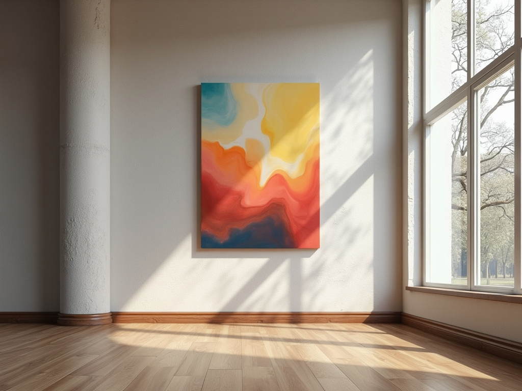
The Problem: Detecting Canvases on Walls
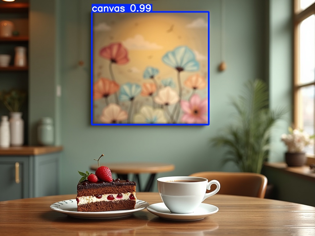
Our goal is to detect canvases on walls in images, determining their exact coordinates within the photo.
Why Fine-tune?
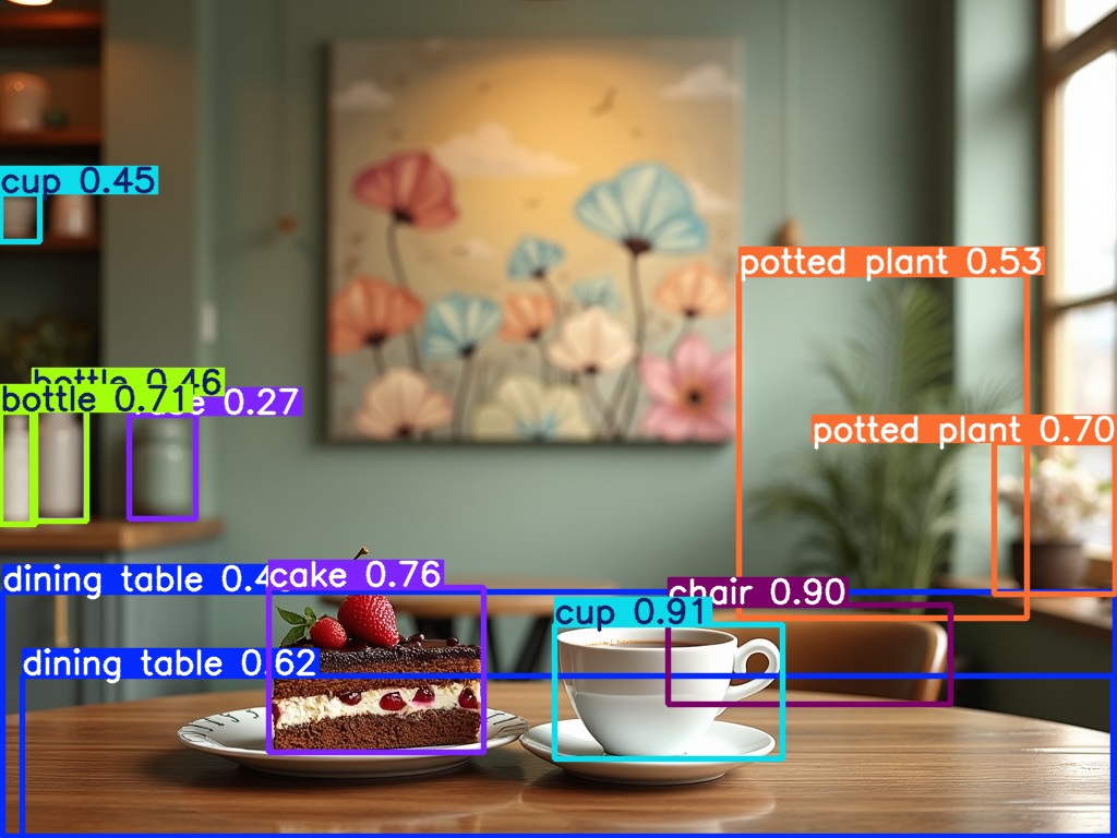
We'll start with a pre-trained YOLO model from Ultralytics as our base. Let's examine this model:
from ultralytics import YOLO

model = YOLO('yolov8n.pt')
print(f"Number of classes: {len(model.names)}")
print(f"Classes: {model.names}")
Output:
Number of classes: 80
Classes: {0: 'person', 1: 'bicycle', 2: 'car', 3: 'motorcycle', 4: 'airplane', 5: 'bus', 6: 'train', 7: 'truck', 8: 'boat', 9: 'traffic light', 10: 'fire hydrant', 11: 'stop sign', 12: 'parking meter', 13: 'bench', 14: 'bird', 15: 'cat', 16: 'dog', 17: 'horse', 18: 'sheep', 19: 'cow', 20: 'elephant', 21: 'bear', 22: 'zebra', 23: 'giraffe', 24: 'backpack', 25: 'umbrella', 26: 'handbag', 27: 'tie', 28: 'suitcase', 29: 'frisbee', 30: 'skis', 31: 'snowboard', 32: 'sports ball', 33: 'kite', 34: 'baseball bat', 35: 'baseball glove', 36: 'skateboard', 37: 'surfboard', 38: 'tennis racket', 39: 'bottle', 40: 'wine glass', 41: 'cup', 42: 'fork', 43: 'knife', 44: 'spoon', 45: 'bowl', 46: 'banana', 47: 'apple', 48: 'sandwich', 49: 'orange', 50: 'broccoli', 51: 'carrot', 52: 'hot dog', 53: 'pizza', 54: 'donut', 55: 'cake', 56: 'chair', 57: 'couch', 58: 'potted plant', 59: 'bed', 60: 'dining table', 61: 'toilet', 62: 'tv', 63: 'laptop', 64: 'mouse', 65: 'remote', 66: 'keyboard', 67: 'cell phone', 68: 'microwave', 69: 'oven', 70: 'toaster', 71: 'sink', 72: 'refrigerator', 73: 'book', 74: 'clock', 75: 'vase', 76: 'scissors', 77: 'teddy bear', 78: 'hair drier', 79: 'toothbrush'}
Now you can see why we need to fine-tune a model for our specific use case. The model is only 6MB in size but doesn't include any class like "canvas", "picture" or "image". This is where fine-tuning comes in handy!
What is Fine-tuning?
Fine-tuning is the process of taking a pre-trained model and adapting it to a new, related task. This approach is beneficial because it:
- Requires less training data than learning from scratch
- Leverages knowledge from the pre-trained model
- Generally results in faster training and better performance
Getting Training Data
In 2024, we can leverage image generation models to create our training data. Using DALL-E 3 and Flux we generated 30 training examples of rooms with canvases on walls.
Labeling Images
We'll use Label Studio for this manual but crucial step:
- Install Label Studio:
uv add label-studio - Start Label Studio:
label-studio -p 8088 - Web brower should open with a link to http://localhost:8088
Using Label Studio is straightforward however if you are doing it for the first time it could be quite confusing, nothing to worry about let's have a look step by step:
- Create an account, this will account on your local instance manageed by you
- Create a new project and choose a project name
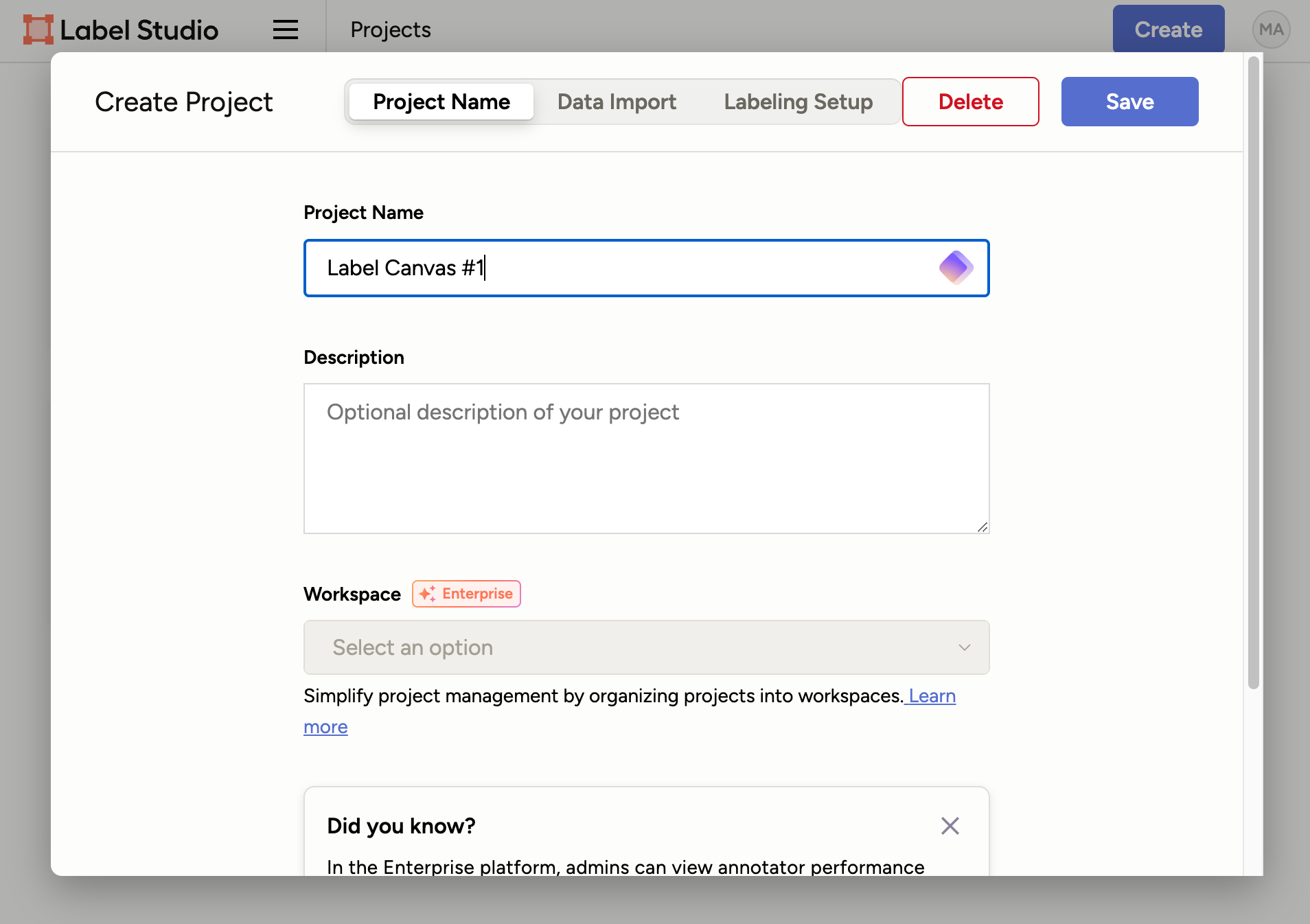
Figure 3: Label Studio - Create a new project - Click on "Data Import", Drag and drop your generated images into the box.
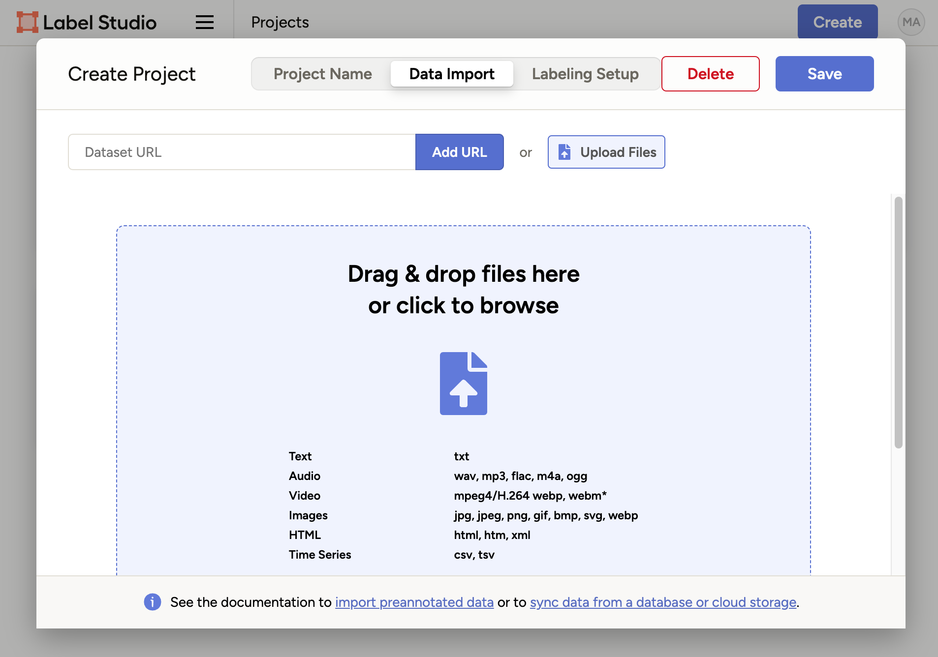
Figure 4: Label Studio - Import data - Now the tricky part. In "Labeling Setup", select "Object detection with bounding boxes"
- Remove the default classes "Airplane" and "Car" by clicking X
- Add a single new class: "canvas" by typing into the input field and clicking "Add", configured
project should look like this:
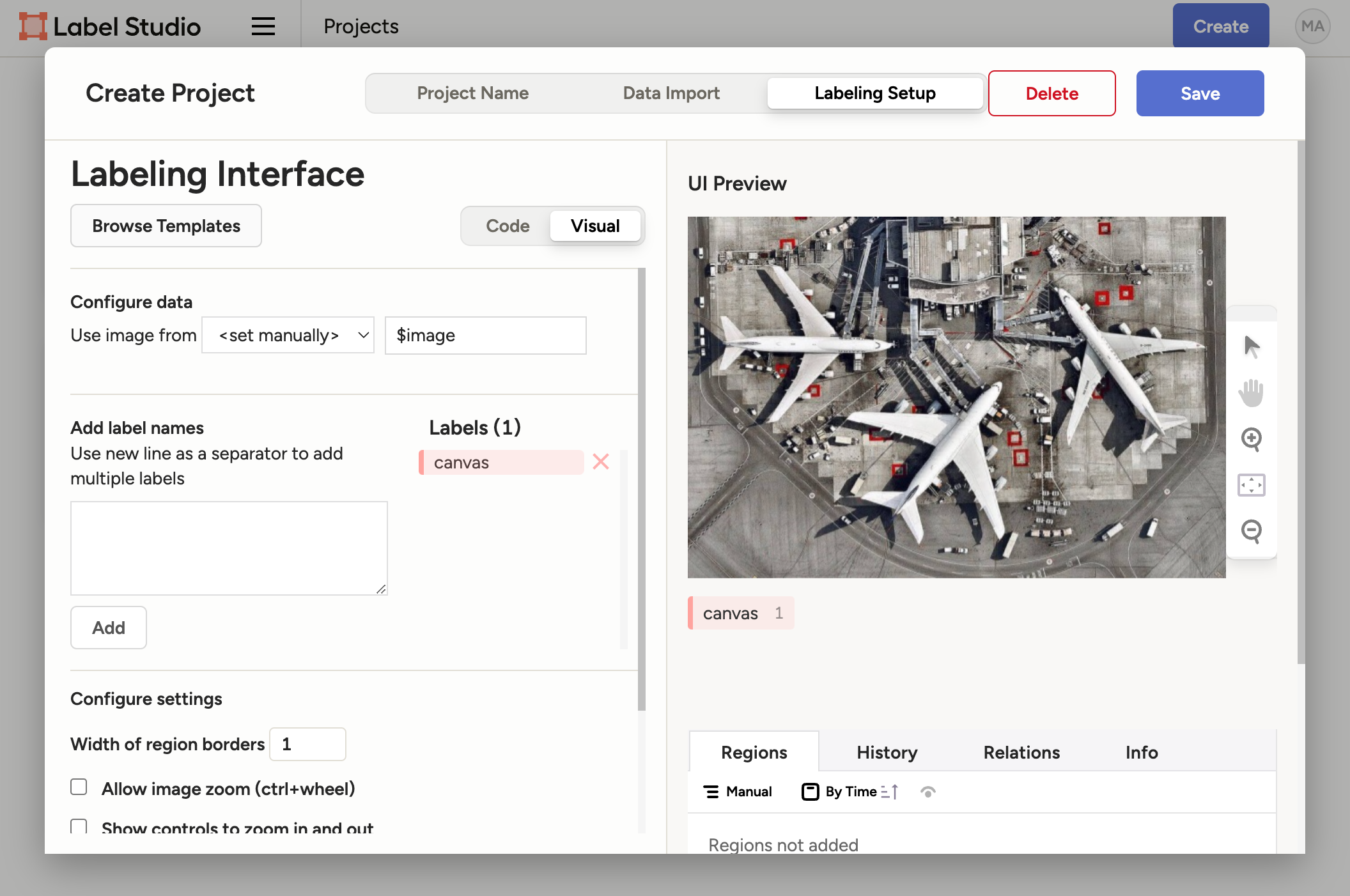
Figure 5: Label Studio - Configured project - Click "Save" to finalize your setup
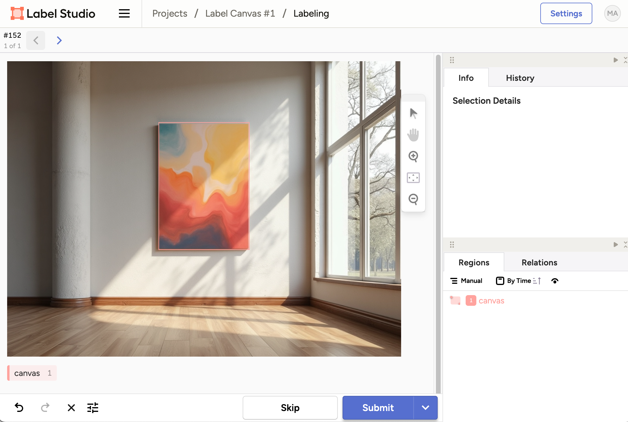
You're now ready to start labeling! Click on "Label All Tasks" to start labeling your data.
As a data scientist, you might be tempted to outsource data labeling. However, especially at the beginning of a project, it's crucial to do this work yourself. It helps you thoroughly understand your data, identify edge cases, and gain valuable insights. Modern labeling interfaces like Label Studio are incredibly efficient, making the process quick and painless.
Pro Tips for Speedy Labeling:
- Press "1" on the keyboard to select the first (and only) class
- Draw the bounding box around the canvas in the image
- Use Command+Enter (or Ctrl+Enter on Windows) to submit and move to the next image
With these shortcuts, you can label your 30 examples quickly and efficiently. Remember, this relatively small dataset is often sufficient for fine-tuning, especially when starting out.
Preparing the Dataset
After labeling, export your data in YOLO format:
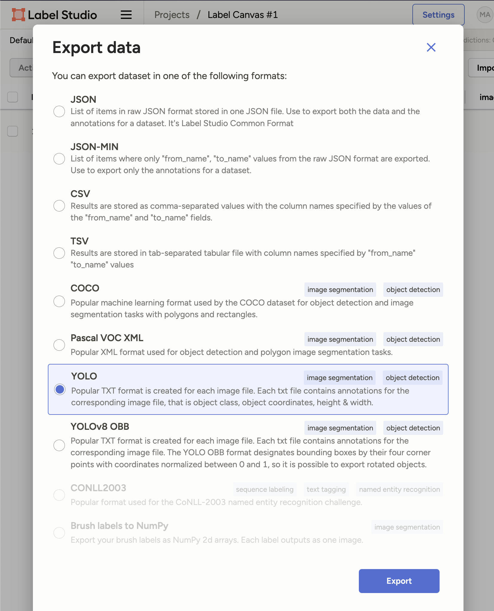
and organize it as follows, it will require copy pasting the images and annotations into the respective folders, you can do this manually or write a simple script to do so:
datasets/
└── canvas/
    ├── train/
    │   ├── images/
    │   └── labels/
    └── val/
        ├── images/
        └── labels/
It is very important to keep train/validation set disjoint, so that you can evaluate the performance of your model on unseen data.
Next step is to create a YAML file (datasets/canvas.yaml) to define your dataset:
path: canvas
train: train
val: val

names:
  0: canvas

hsv_h: .015
hsv_s: .7
hsv_v: .4
translate: .3
scale: .5
shear: .01
flipud: .3
fliplr: .5
mixup: .5
auto_augment: randaugment
Let's briefly explain the YOLO parameters in the YAML file:
path,train,val: Define the dataset structure and splitsnames: Lists the class names (in our case, just "canvas")hsv_h,hsv_s,hsv_v: Control color augmentationtranslate,scale,shear: Geometric transformations for data augmentationflipud,fliplr: Probabilities for vertical and horizontal flippingmixup: Probability of applying mixup augmentationauto_augment: Specifies the automatic augmentation policy
These parameters help in creating a robust model by introducing variability in the training data.
Training the Model
Now for the exciting part - training our model! On a MacBook with M1 chip:
yolo train data=datasets/canvas.yaml device=mps
For GPU users:
yolo train data=datasets/canvas.yaml device=cuda
Results and Model Performance
After training, check the "runs/detect" folder for detailed reports and visualizations. The best model will be in "weights/best.pt".
Training Performance
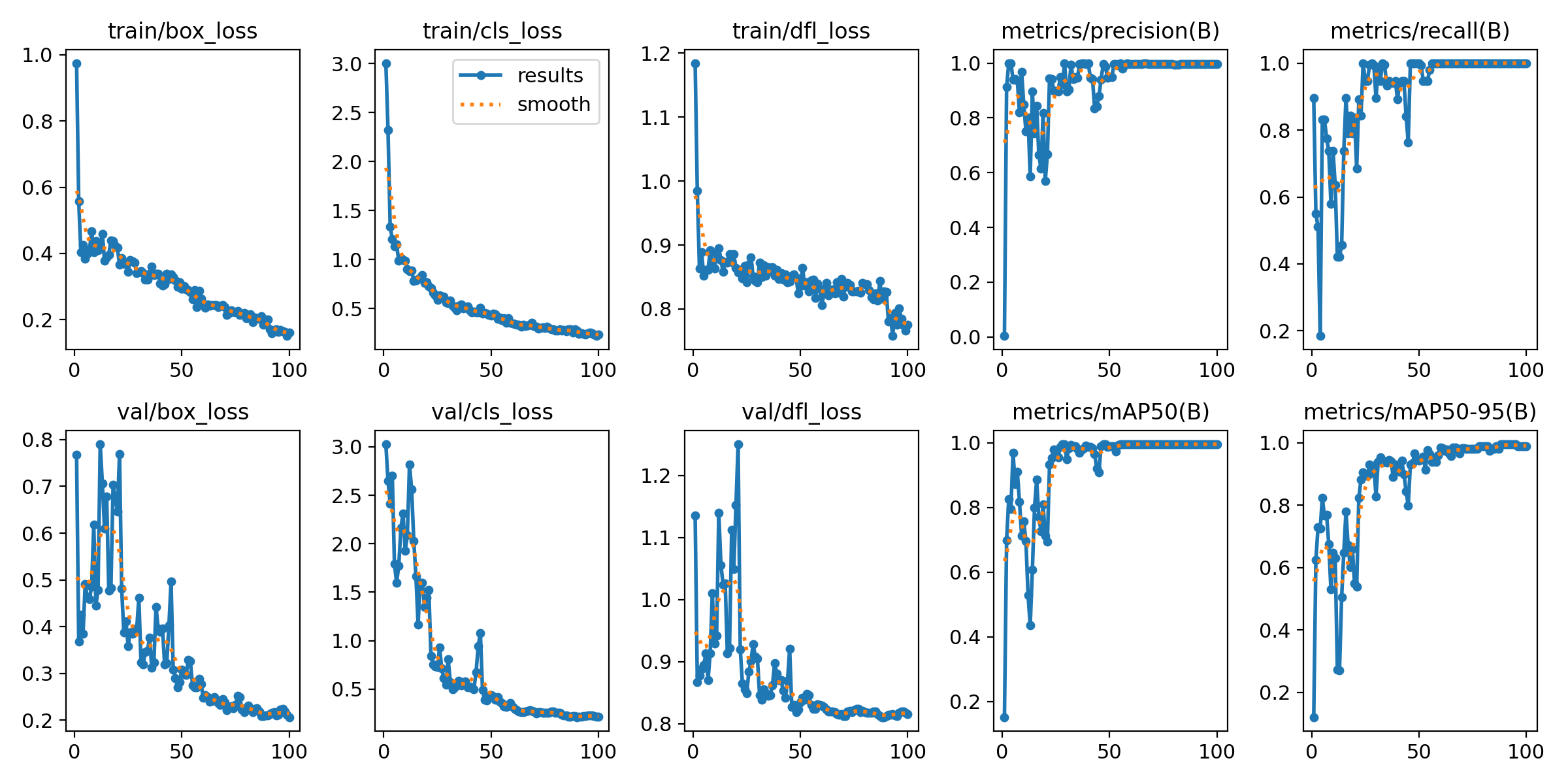
In our run, the model achieved a training mAP of 0.995, which is essentially perfect for our use case.
Understanding Model Evaluation Metrics
We mentioned achieving a mAP (mean Average Precision) of 0.995. Here's what that means:
- mAP is a standard metric for object detection tasks
- It ranges from 0 to 1, with 1 being perfect detection
- Our score of 0.995 indicates excellent performance on our dataset
However, it's crucial to test the model on diverse, real-world images to ensure its generalization ability.
Making Predictions
To make predictions, we'll use the following code:
model = YOLO("runs/detect/train/weights/best.pt")
print(model.names)
results = model(["object_detection.jpg"])

# Process results list
for result in results:
    boxes = result.boxes  # Boxes object for bounding box outputs
    masks = result.masks  # Masks object for segmentation masks outputs
    keypoints = result.keypoints  # Keypoints object for pose outputs
    probs = result.probs  # Probs object for classification outputs
    obb = result.obb  # Oriented boxes object for OBB outputs
    result.show()  # display to screen
    result.save(filename="result.jpg")  # save to disk
Conclusion
We've successfully fine-tuned a YOLO model to detect canvases on walls, achieving high accuracy with just 30 training examples. The resulting model is only 6.3MB in size and can run in real-time on a phone, demonstrating the power and efficiency of YOLO for custom object detection tasks.
Challenges and Limitations
While our approach is effective, it's important to be aware of potential challenges:
- The small dataset (30 images) may not be sufficient for more complex tasks
- There's a risk of overfitting with such a limited dataset
- Using synthetic data for training may not fully represent real-world scenarios
Next Steps
- Experiment with different augmentation techniques
- Try fine-tuning for other custom objects
- Explore deployment options for mobile and web applications